Time Analysis
You can create a simple time analysis of a classified trajectory by using the transition submodule
The time analysis works with the concepts of windows and stride.
The window is the number of frame between wich the state of an atom is confronted, the more is higher the window the more time passes between the two states: 
The stride is how many frames the window with the confronatation is displaced during the analysis. A stride must be alwayis inferior or equal to the value of the window: 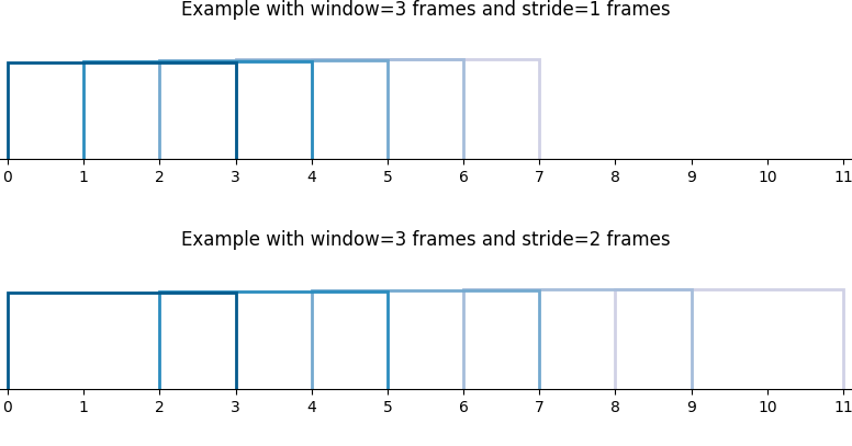
If you want to analyze the trajectory as if it has been sampled at a slower rate simply use the same number for window and stride: 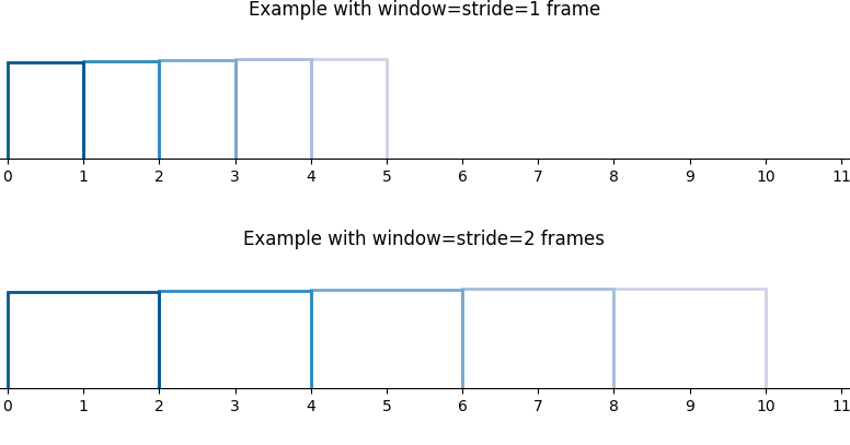
[1]:
import numpy.random as npr
import numpy as np
from scipy.stats import poisson, kstest, norm
from scipy.optimize import curve_fit
import matplotlib.pyplot as plt
import SOAPify.transitions as st
from SOAPify import SOAPclassification
import seaborn as sns
[2]:
rng = npr.default_rng(12345)
cls=SOAPclassification(
    [],
    rng.integers(0, 3, size=(500,1)),
    [0,1,2]
    )
_,ax=plt.subplots(figsize=(10,3))
ax.set_yticks([0,1,2])
_ =ax.plot(cls.references[:,0])

[3]:
tmat = st.calculateTransitionMatrix(cls)
tmat= st.normalizeMatrix(tmat)
sns.heatmap(tmat, annot=True,linewidths=0.1,square=True,vmax=1, vmin=0)
[3]:
<AxesSubplot: >

Example: a 4 states Markov chain
A simple 1 atom system with 4 states and possibility to evolve only to adiacent states
[4]:
rng = npr.default_rng(123456)
nframes=1000
P=np.array([
    [0.8,0.2,0.0,0.0],
    [0.1,0.7,0.2,0.0],
    [0.0,0.3,0.6,0.1],
    [0.0,0.0,0.2,0.8],
            ])
#contstuct a target table:
target=P
for j in range(1,4):
    target[:,j]+=target[:,j-1]


cls=np.empty((nframes,1),dtype=int)
cls[0,0]=1
for i,c in enumerate(cls[:-1,0]):
    t=rng.random()
    cls[i+1,0]= np.argwhere(target[c]>t)[0]
cls=SOAPclassification(
    [],
    cls,
    [0,1,2,3]
    )
_,axes=plt.subplots(2,1,figsize=(12,6))
for ax in axes:
    ax.set_yticks([0,1,2,3])

axes[0].plot(cls.references[:,0])
axes[0].set_title("The whole trajectory")
axes[1].set_title("The first 50 steps sampled at 1,2, and 5 frames")
for window in [1,2,5]:
    axes[1].plot(np.arange(0,51,window),
            cls.references[:51:window,0],marker=window+1,
            label=f"simulation sampled at window={window}")
_=axes[1].legend()

The transition matrices calculated changing the window value and the stride value
[5]:
_,ax=plt.subplots(2,4,figsize=(10,6), gridspec_kw={'width_ratios':[1,1,1,0.1]})
for i, window in enumerate([1,2,5]):
    tmat = st.calculateTransitionMatrix(cls, window=window, stride=1)
    tmat= st.normalizeMatrix(tmat)
    sns.heatmap(tmat, annot=True,linewidths=0.1,
                square=True,vmax=1, vmin=0, ax = ax[0,i],
                cbar=i != 1,
                cbar_ax= ax[0,3] if i!=1  else None)
    ax[0,i].set_title(f"window={window}, stride=1")
for i, window in enumerate([1,2,5]):
    tmat = st.calculateTransitionMatrix(cls, window=window, stride=window)
    tmat= st.normalizeMatrix(tmat)
    sns.heatmap(tmat, annot=True,linewidths=0.1,
                square=True,vmax=1, vmin=0, ax = ax[1,i],
                cbar=i != 1,
                cbar_ax= ax[1,3] if i!=1  else None)
    ax[1,i].set_title(f"window=stride={window}")

How to calculate and show the events
calculateResidenceTimes creates a list of residence time for each state of the given trajectory. The algorithm will set the first and last residence time with a negative time, to suggest that these event are not correctly sampled.
[6]:
residenceTimes = st.calculateResidenceTimes(
        cls, stride=1, window=1
    )
_,ax=plt.subplots(figsize=(12,6))
for i,RT in enumerate(residenceTimes):
    completeRT=RT[RT>0]
    nOfCounts=len (completeRT)
    uniqueElements, counts=np.unique(completeRT,return_counts=True)
    for j in range(1,len(counts)):
        counts[j]+=counts[j-1]
    ax.step(uniqueElements, counts/nOfCounts,
            where='post',label = f"state {i}",
            marker='x', color=f"C{i}")
    #ys=(np.array(range(len (completeRT)))+1)/(len (completeRT))
    #ax.plot(completeRT, ys, label = f"state {i}", marker='o',color=f"C{i}")
ax.set_xlabel("Nof frames")
_=ax.legend()

You can estimate the transition time by fitting a cumulative distribution function against the cumulative of the points, and then by testing the correctness with a Kolmogorov-Smirnov test.
Here we are using a Poissonian as an example distribution.
[7]:
_,axes=plt.subplots(2,2,figsize=(12,6))
ax= axes.flatten()
xs= np.arange(np.amax([np.amax(RT) for RT in residenceTimes])+1)

for i,RT in enumerate(residenceTimes):
    completeRT=RT[RT>0]
    nOfCounts=len (completeRT)
    uniqueElements, counts=np.unique(completeRT,return_counts=True)
    for j in range(1,len(counts)):
        counts[j]+=counts[j-1]
    counts=counts/nOfCounts
    ax[i].step(uniqueElements,counts , where='post',label = f"state {i}",
            marker='x', color=f"C{i}")
    mu,_=curve_fit(poisson.cdf,uniqueElements,counts, p0=[1])
    ks=kstest(completeRT,poisson.cdf(xs,mu))
    ax[i].step(xs,poisson.cdf(xs,mu),where='post', color=f"C{i}",
            linestyle='--',
            label=f'bestfit for "{i}": mu={mu[0]:0.4g}\n statistic={ks[0]:.2g} p={ks[1]:.2g}')

    ax[i].set_xlabel("Nof frames")
    ax[i].legend()

And here we are using a normal as an example distribution
[8]:
_,axes=plt.subplots(2,2,figsize=(12,6))
ax= axes.flatten()
xs= np.arange(np.amax([np.amax(RT) for RT in residenceTimes])+1)

for i,RT in enumerate(residenceTimes):
    completeRT=RT[RT>0]
    nOfCounts=len (completeRT)
    uniqueElements, counts=np.unique(completeRT,return_counts=True)
    for j in range(1,len(counts)):
        counts[j]+=counts[j-1]
    counts=counts/nOfCounts
    ax[i].step(uniqueElements,counts , where='post',label = f"state {i}",
            marker='x', color=f"C{i}")
    mu,_=curve_fit(norm.cdf,uniqueElements,counts, p0=[1,1])
    ks=kstest(completeRT,norm.cdf(xs,mu[0], mu[1]))
    ax[i].step(xs,norm.cdf(xs,mu[0], mu[1]),where='post', color=f"C{i}",
            linestyle='--',
            label=f'bestfit for "{i}": sigma={mu[0]:0.4g}\n statistic={ks[0]:.2g} p={ks[1]:.2g}')

    ax[i].set_xlabel("Nof frames")
    ax[i].legend()
