timeSOAP analysis
an example for a timeSOAP analysis as in the original paper
[1]:
import SOAPify.HDF5er as HDF5er
from SOAPify import (
    saponifyTrajectory,
    fillSOAPVectorFromdscribe,
    normalizeArray,
    getSOAPSettings,
)
from SOAPify.analysis import timeSOAPsimple
import h5py
import matplotlib.pyplot as plt
from matplotlib.collections import LineCollection
from matplotlib.patches import Circle
from matplotlib.colors import ListedColormap, BoundaryNorm
from scipy.signal import savgol_filter
from sklearn.cluster import KMeans
from sklearn.metrics import silhouette_score
import numpy as np
from multiprocessing.pool import ThreadPool as Pool
from seaborn import kdeplot

SOAPrcut = 4.48023312
SOAPnmax = 8
SOAPlmax = 8
Load data
Let’s get the data:
wget https://github.com/GMPavanLab/dynNP/releases/download/V1.0-trajectories/ico309.hdf5
We’ll start by caclulating the SOAP fingerprints of the 500 K simulation
using lMax=8, nMax=8, and cutoff=4.48023312 that is 10% more than the Au cell
[2]:
trajFileName = "ico309.hdf5"
trajAddress = "ico309-SV_18631-SL_31922-T_500"
[3]:
def prepareSOAP(trajFileName, trajAddress):
    soapFileName = trajFileName.split(".")[0] + "soap.hdf5"
    print(trajFileName, soapFileName)
    with h5py.File(trajFileName, "r") as workFile, h5py.File(
        soapFileName, "a"
    ) as soapFile:
        soapFile.require_group("SOAP")
        # skips if the soap trajectory is already present
        if trajAddress not in soapFile["SOAP"]:
            saponifyTrajectory(
                trajContainer=workFile[f"Trajectories/{trajAddress}"],
                SOAPoutContainer=soapFile["SOAP"],
                SOAPOutputChunkDim=1000,
                SOAPnJobs=32,
                SOAPrcut=SOAPrcut,
                SOAPnmax=SOAPnmax,
                SOAPlmax=SOAPlmax,
            )
    return soapFileName


soapFileName = prepareSOAP(trajFileName, trajAddress)
ico309.hdf5 ico309soap.hdf5
Let’s get the raw tempSOAP array without clogging up the memory
There is an improved version of the action in shis cell in the analysis submodule: analysis.getTimeSOAPSimple
[4]:
def getTimeSOAP(soapFileName, trajAddress):
    with h5py.File(soapFileName, "r") as f:
        ds = f[f"/SOAP/{trajAddress}"]
        fillSettings = getSOAPSettings(ds)
        print(fillSettings)
        print(ds.shape)
        nAt = ds.shape[1]

        timedSOAP = np.zeros((ds.shape[0] - 1, ds.shape[1]))

        print(timedSOAP.shape)
        slide = 0
        # this looks a lot convoluted, but it is way faster than working one atom
        # at a time
        for c in ds.iter_chunks():
            theSlice = slice(c[0].start - slide, c[0].stop, c[0].step)
            outSlice = slice(c[0].start - slide, c[0].stop - 1, c[0].step)
            print(c[0], theSlice, outSlice)
            timedSOAP[outSlice], _ = timeSOAPsimple(
                normalizeArray(fillSOAPVectorFromdscribe(ds[theSlice], **fillSettings))
            )
            slide = 1

        return nAt, timedSOAP, np.diff(timedSOAP.T, axis=-1)


nAtoms, tSOAP, dtSOAP = getTimeSOAP(soapFileName, trajAddress)
{'nMax': 8, 'lMax': 8, 'atomTypes': array(['Au'], dtype=object), 'atomicSlices': {'AuAu': slice(0, 324, None)}}
(20000, 309, 324)
(19999, 309)
slice(0, 1000, 1) slice(0, 1000, 1) slice(0, 999, 1)
slice(1000, 2000, 1) slice(999, 2000, 1) slice(999, 1999, 1)
slice(2000, 3000, 1) slice(1999, 3000, 1) slice(1999, 2999, 1)
slice(3000, 4000, 1) slice(2999, 4000, 1) slice(2999, 3999, 1)
slice(4000, 5000, 1) slice(3999, 5000, 1) slice(3999, 4999, 1)
slice(5000, 6000, 1) slice(4999, 6000, 1) slice(4999, 5999, 1)
slice(6000, 7000, 1) slice(5999, 7000, 1) slice(5999, 6999, 1)
slice(7000, 8000, 1) slice(6999, 8000, 1) slice(6999, 7999, 1)
slice(8000, 9000, 1) slice(7999, 9000, 1) slice(7999, 8999, 1)
slice(9000, 10000, 1) slice(8999, 10000, 1) slice(8999, 9999, 1)
slice(10000, 11000, 1) slice(9999, 11000, 1) slice(9999, 10999, 1)
slice(11000, 12000, 1) slice(10999, 12000, 1) slice(10999, 11999, 1)
slice(12000, 13000, 1) slice(11999, 13000, 1) slice(11999, 12999, 1)
slice(13000, 14000, 1) slice(12999, 14000, 1) slice(12999, 13999, 1)
slice(14000, 15000, 1) slice(13999, 15000, 1) slice(13999, 14999, 1)
slice(15000, 16000, 1) slice(14999, 16000, 1) slice(14999, 15999, 1)
slice(16000, 17000, 1) slice(15999, 17000, 1) slice(15999, 16999, 1)
slice(17000, 18000, 1) slice(16999, 18000, 1) slice(16999, 17999, 1)
slice(18000, 19000, 1) slice(17999, 19000, 1) slice(17999, 18999, 1)
slice(19000, 20000, 1) slice(18999, 20000, 1) slice(18999, 19999, 1)
[5]:
print(tSOAP.shape)
print(dtSOAP.shape)
(19999, 309)
(309, 19998)
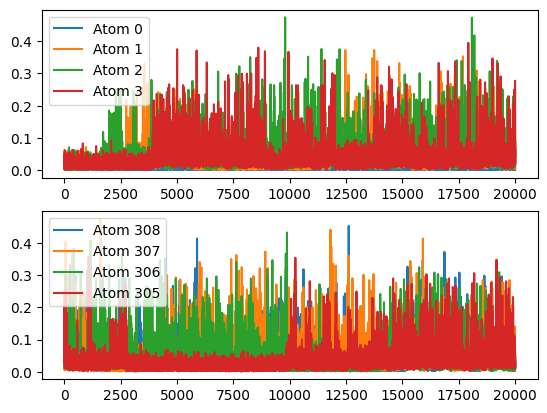
[6]:
fig, axes = plt.subplots(2, sharey=True)
for i in range(4):
    axes[0].plot(tSOAP[:, i], label=f"Atom {i}")
    axes[1].plot(tSOAP[:, nAtoms - 1 - i], label=f"Atom {nAtoms-1-i}")

for ax in axes:
    ax.legend()
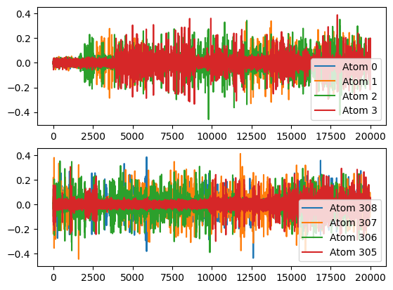
[7]:
fig, axes = plt.subplots(2, sharey=True)
for i in range(4):
    axes[0].plot(dtSOAP[i], label=f"Atom {i}")
    axes[1].plot(dtSOAP[308 - i], label=f"Atom {308-i}")

for ax in axes:
    ax.legend()
Filtering
Let’s chose an atom try to apply a filter on it. We want try to reduce the signal to noise ratio, so we calculate the mean of the s/n for all atoms:
[8]:
def signaltonoise(a: np.array, axis, ddof):
    """Given an array, retunrs its signal to noise value of its compontens"""
    m = a.mean(axis)
    sd = a.std(axis=axis, ddof=ddof)
    return 20 * np.log10(abs(np.where(sd == 0, 0, m / sd)))
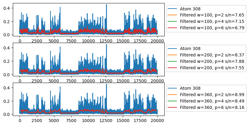
Here we show the effect of the savitszky-golay filtering on the last atom. In the legend we show the mean (on all the atoms) signal to noise ration (s/n).
[9]:
atom = nAtoms - 1
savGolPrint = np.arange(tSOAP.T[atom].shape[0])
windows = [100, 200, 360]
polyorders = [2, 4, 6]
fig, axes = plt.subplots(len(windows), sharey=True)

for ax, window_length in zip(axes, windows):
    windowToPlot = slice(window_length // 2, -window_length // 2)
    ax.plot(tSOAP.T[atom], label=f"Atom {atom}")
    for polyorder in polyorders:
        savgol = savgol_filter(
            tSOAP.T, window_length=window_length, polyorder=polyorder, axis=-1
        )

        sr_ratio = signaltonoise(savgol[:, windowToPlot], axis=-1, ddof=0)

        ax.plot(
            savGolPrint[windowToPlot],
            savgol[atom, windowToPlot],
            label=f"Filtered w={window_length}, p={polyorder} s/n={np.mean(sr_ratio):.2f}",
        )
    ax.legend(loc="upper left", bbox_to_anchor=(1, 1))
Here we show the evolution of the mean s/n ratio with the change in the parameters of the savitszky-golay for these signals
[10]:
windows = np.arange(10, 600, 20)
polyorders = [2, 4, 6]
fig, ax = plt.subplots(1)


for polyorder in polyorders:
    meansrRatios = np.empty((len(windows), 2))
    for i, window_length in enumerate(windows):
        windowToPlot = slice(window_length // 2, -window_length // 2)
        savgol = savgol_filter(
            tSOAP.T, window_length=window_length, polyorder=polyorder, axis=-1
        )
        sr_ratio = signaltonoise(savgol[:, windowToPlot], axis=-1, ddof=0)
        meansrRatios[i] = [window_length, np.mean(sr_ratio)]
    ax.plot(meansrRatios[:, 0], meansrRatios[:, 1], label=f"p={polyorder}")
ax.set_xlabel("Window Size", fontsize=20)
ax.set_ylabel("S/N [dB]", fontsize=20)

_ = ax.legend()
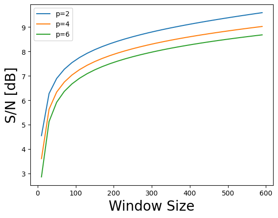
We proceed with window_length=360 and polyorder=2, it as a 8.99 dB signal to noise ratio, that is quite accettable,
with these parameters we have a good compromise between the window and the s/n ration
[11]:
window_length = 360
polyorder = 2
windowToUSE = slice(window_length // 2, -window_length // 2)
filteredtSOAP = savgol_filter(
    tSOAP.T, window_length=window_length, polyorder=polyorder, axis=-1
)
We chose to execute a K-Means clustering oh the values of the signals, using 5 as the number of clusters
[12]:
bestnclusters = 5
clusters = KMeans(bestnclusters, random_state=12345).fit_predict(
    filteredtSOAP.reshape(-1, 1)
)
data_KM = {}
for i in range(bestnclusters):
    data_KM[i] = {}
    data_KM[i]["elements"] = filteredtSOAP.reshape((-1))[clusters == i]
    data_KM[i]["min"] = np.min(data_KM[i]["elements"])
    data_KM[i]["max"] = np.max(data_KM[i]["elements"])
[13]:
fig, axes = plt.subplots(
    1, 2, figsize=(6, 3), dpi=200, width_ratios=[3, 1.2], sharey=True
)

for flns in filteredtSOAP:
    axes[0].plot(
        savGolPrint[windowToUSE],
        flns[windowToUSE],
        color="k",
        linewidth=0.01,
        # alpha=0.9,
    )
hist = axes[1].hist(
    filteredtSOAP.reshape((-1)),
    alpha=0.7,
    color="gray",
    bins="doane",
    density=True,
    orientation="horizontal",
)
kde = kdeplot(
    y=filteredtSOAP.reshape((-1)),
    bw_adjust=1.5,
    linewidth=2,
    color="black",
    # gridsize=500,
    gridsize=2 * (hist[1].shape[0] - 1),
    ax=axes[1],
)
axes[0].set_title('tSOAP "trajectories"')
axes[0].set_xlim(0, len(savGolPrint))
axes[1].set_title("Density of\ntSOAP values")
height = np.max(hist[0])
for cname, data in data_KM.items():
    # center = delta+data['min']
    bin_size = data["max"] - data["min"]
    for i, ax in enumerate(axes):
        ax.barh(
            y=data["min"],
            width=len(savGolPrint) if i == 0 else height,
            height=bin_size,
            align="edge",
            alpha=0.25,
            # color=colors[idx_m],
            linewidth=2,
        )
        ax.axhline(y=data["min"], c="red", linewidth=2, linestyle=":")
        if i == 1:
            ax.text(
                -0.25,
                data["min"] + bin_size / 2.0,
                f"c{cname}",
                va="center",
                ha="right",
                fontsize=18,
            )

The idea is to play with the clustering until you are satisfied, then to visualize and try to give an interpretation (and then change agani the method of clustering until you are satisfied):
Visualization: ovito-compatible
Let’s define some helper functions and then export the data in a xyz that is compatible with ovito
[14]:
def prepareData(x, /):
    """prepares an array from shape (atom,frames) to  (frames,atom)"""
    shape = x.shape
    toret = np.empty((shape[1], shape[0]), dtype=x.dtype)
    for i, atomvalues in enumerate(x):
        toret[:, i] = atomvalues
    return toret


# classyfing by knoing the min/max of the clusters
def classifying(x, classDict):
    toret = np.ones_like(x, dtype=int) * (len(classDict) - 1)
    # todo: sort  by max and then classify
    minmax = [[cname, data["max"]] for cname, data in data_KM.items()]
    minmax = sorted(minmax, key=lambda x: -x[1])
    # print(minmax)
    for cname, myMax in minmax:
        toret[x < myMax] = int(cname)
    return toret


classifiedFilteredtSOAP = classifying(filteredtSOAP, data_KM)
[15]:
def export(trajFileName, trajAddress):
    # as a function, so the universe should be garbage collected correctly
    with h5py.File(trajFileName, "r") as trajFile, open(
        "outClassifiedTimeSOAP.xyz", "w"
    ) as xyzFile:
        from MDAnalysis.transformations import fit_rot_trans

        wantedTrajectory = slice(-1)

        tgroup = trajFile[f"/Trajectories/{trajAddress}"]
        universe = HDF5er.createUniverseFromSlice(tgroup, wantedTrajectory)
        nAt= len(universe.atoms)
        universe.add_TopologyAttr("mass", [1] * nAt)
        ref = HDF5er.createUniverseFromSlice(tgroup, [0])
        ref.add_TopologyAttr("mass", [1] * nAt)
        universe.trajectory.add_transformations(fit_rot_trans(universe, ref))

        HDF5er.getXYZfromMDA(
            xyzFile,
            universe,
            allFramesProperty='Origin="-40 -40 -40"',
            tSOAP=tSOAP,
            filteredtSOAP=prepareData(filteredtSOAP),
            proposedClassification=prepareData(classifiedFilteredtSOAP),
        )


export(trajFileName, trajAddress)
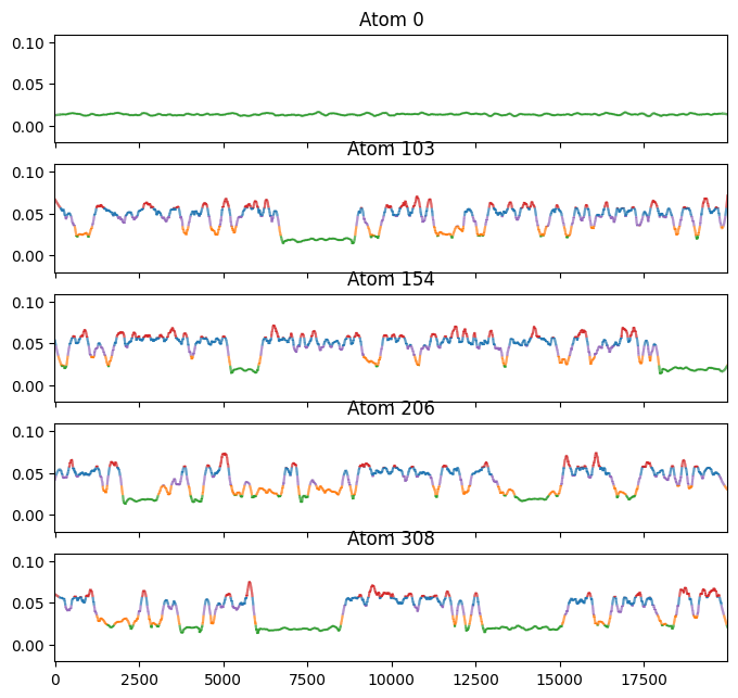
Let’s visualize a few tSOAP trajectories colored by the cluster in time
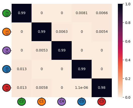
Time analysis and visualizations
Let’s calculate the transition matrix for this tSOAP analysis
[16]:
minmax = [[cname, data["max"]] for cname, data in data_KM.items()]
minmax = sorted(minmax, key=lambda x: x[1])
cmap = ListedColormap([f"C{m[0]}" for m in minmax])
norm = BoundaryNorm([0] + [m[1] for m in minmax], cmap.N)
[17]:
from SOAPify import SOAPclassification, calculateTransitionMatrix, normalizeMatrixByRow
from seaborn import heatmap

classifications = SOAPclassification(
    [], prepareData(classifiedFilteredtSOAP), [f"C{m[0]}" for m in minmax]
)
tmat = calculateTransitionMatrix(classifications)
tmat = normalizeMatrixByRow(tmat)
_, ax = plt.subplots(1)
heatmap(
    tmat,
    vmax=1,
    vmin=0,
    cmap="rocket_r",
    annot=True,
    xticklabels=classifications.legend,
    yticklabels=classifications.legend,
    ax=ax,
)

for i, label in enumerate(classifications.legend):
    ax.add_patch(
        Circle(
            (0.5 + i, len(classifications.legend) + 0.25),
            facecolor=label,
            lw=1.5,
            edgecolor="black",
            radius=0.2,
            clip_on=False,
        )
    )
    ax.add_patch(
        Circle(
            (-0.25, 0.5 + i),
            facecolor=label,
            lw=1.5,
            edgecolor="black",
            radius=0.2,
            clip_on=False,
        )
    )
[18]:
chosenAtoms=[0, nAtoms //3,nAtoms//2,int(nAtoms//3)*2, nAtoms - 1]
fig, axes = plt.subplots(len(chosenAtoms),figsize=(8,1.5*len(chosenAtoms)), sharey=True, sharex=True)

for atom, ax in zip(chosenAtoms, axes):
    points = np.array([savGolPrint, filteredtSOAP[atom]]).T.reshape(-1, 1, 2)
    segments = np.concatenate([points[:-1], points[1:]], axis=1)
    lc = LineCollection(segments, cmap=cmap, norm=norm)
    lc.set_array(filteredtSOAP[atom])

    line = ax.add_collection(lc)
    ax.set_title(f"Atom {atom}")

axes[0].set_xlim(savGolPrint[0] - 1, savGolPrint[-1] + 1)
_ = axes[0].set_ylim(-0.02, np.max(filteredtSOAP) + 0.02)